
GeniusTrader will output data in a few different formats depending on the nature of the command being used and the options specified. For the most part chart images are just that, image files, however, some GT script apps will output as ascii text and or html. For details review the specific GT script app man page (pod) or built-in help.
Unfortunately, GT does not provide the sample price data
used all of these examples but there is a limited amount of
sample data available here.
Unroll the sample data tarball in the directory just above your
GeniusTrader Scripts dir.
So if the curent working directory (cwd) is Scripts,
the parent dir hierarchy,
when listed, might look like this:
$ ls -F ..
  GT/                   Scripts/              sample_data/
  website/
Note the colors used above -- command lines you will be
typing are shown like this, the terminal output
will be shown like this.
     a large block of indented text like this.
     please enter this text into a file usually named
     in the command line immediately above it.


     the file name will be something along the lines
     of screenshot_x.gconf, or something.scan
If you do try to generate the charts shown here you should expect the images to vary slightly depending on the set of price data you are using, your specific $HOME/.gt/options file which sets colors for the various graphic objects (candles, volume histogram, regular histogram, etc), that may differ from that used to generate these images, defines the graphic image type to be generated (e.g. png, svg, postscript, imagemagick) and associates your platforms available fonts to the font names GT uses.
See the First time tutorial to ensure your GT setup and configuration is basically working.
graphic.pl
is used to create the Screen Shot 1 image using
this command line:
$ ./graphic.pl --file screenshot_1.gconf --out 'Screenshot 1.png' IBM
where the output image will be written on file
Screenshot 1.png
and the graphic directives read from file screenshot_1.gconf
which contains these lines
    #
    # ./graphic.pl --file screenshot_1.gconf --out 'Screenshot 1.png' IBM
    #
    --start=2003-08-01
    --end=2004-02-01
    --timeframe=day
    --title=ScreenShot 1: %c
    --type=candle
    --add=MountainBand(Indicators::BOL/2 20 2.0,Indicators::BOL/3 15 2.0, \
      [160,160,0,100])
    --add=Curve(Indicators::SMA 100, [0,0,0])
    --add=Curve(Indicators::SMA 20, [0,0,255])
    --add=Curve(Indicators::SMA 5, [255,0,0])
    --add=VotingLine( Systems::Generic \
      { S:Generic:Above {I:Prices CLOSE} {I:BOL/2 20 2.0} } \
      { S:Generic:Below {I:Prices CLOSE} {I:BOL/3 15 2.0} }, 4 )
    --add=New-Zone(6)
    --add=New-Zone(75)
    --add=Histogram(Indicators::MACD/3,lightblue)
    --add=Curve(Indicators::MACD,[0,0,255])
    --add=Curve(Indicators::MACD/2,[255,0,0])
    --add=Text(MACD, 50, 50, center, center, giant, [80,160,240,70], times)
    --add=New-Zone(6)
    --add=New-Zone(75)
    --add=Curve(Indicators::ADX/4,[0,0,128])
    --add=Curve(Indicators::ADX/1,[0,128,0])
    --add=Curve(Indicators::ADX/2,[199,199,199])
    --add=Curve(Indicators::ADX/3,[128,0,0])
    --add=MountainBand(Indicators::Generic::Eval \
      0,Indicators::Generic::Eval \
      min(20,{Indicators::ADX/4}),[128,128,0,100])
    --add=MountainBand(Indicators::Generic::Eval \
      min(20,{Indicators::ADX/4}),Indicators::ADX/4,[228,128,0,100])
    --add=Curve(Indicators::Generic::Eval 20,[0,0,255])
    --add=Text(ADX, 50, 50, center, center, giant, [80,160,240,70], times)
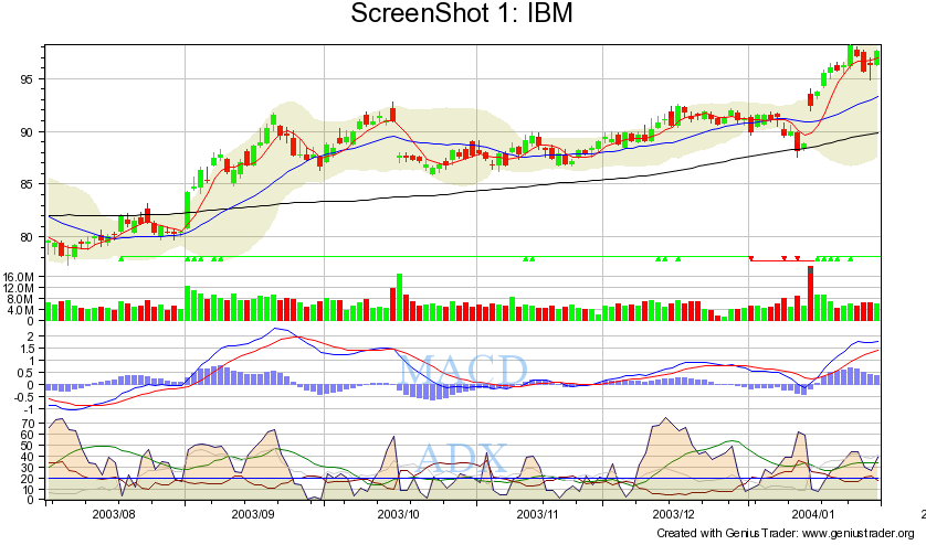
This first screen shot depicts a day timeframe
candle price chart (the default) overlayed with three SMA curves and a
Bollinger Band envelope with different parameters for each boundary.
This chart also shows a VotingLine based on the Bollinger Band envelope.
The volume and two additional indicator plots,
MACD and ADX are also plotted. The ADX plot shows how to
use the MountainBand graphic object to do multi-color fills.
Screen Shot 2 was created using the following
graphic.plcommand:
$ ./graphic.pl --file screenshot_2.gconf --out 'Screenshot 2.png' VOD
where the graphic directives file screenshot_2.gconf
contains these lines
    #
    # ./graphic.pl --file screenshot_2.gconf --out 'Screenshot 2.png' VOD
    #
    --start=2003-09-01
    --end=2004-03-01
    --title=ScreenShot 2: %n
    --type=candlevolplace
    --add=Curve(Indicators::KAMA, [255,0,0])
    --add=Text(KAMA, 10, 90, center, center, small, [255,0,0], times)
    --add=BuySellArrows(Systems::Generic \
      { S::Generic::CrossOverUp   {I:Prices CLOSE} {I:KAMA} } \
      { S::Generic::CrossOverDown {I:Prices CLOSE} {I:KAMA} } )

    --add=New-Zone(6)
    --add=New-Zone(100)
    --add=MountainBand(Indicators::Generic::If \
      {S:Generic:Above {I:RSI} 70} \
      {I:RSI} 70,Indicators::Generic::Eval 70,[255,0,0,90])
    --add=MountainBand(Indicators::Generic::If \
      {S:Generic:Below {I:RSI} 30} \
      {I:RSI} 30,Indicators::Generic::Eval 30,[0,255,0,90])
    --add=Curve(Indicators::RSI)
    --add=Curve(Indicators::Generic::Eval 70)
    --add=Curve(Indicators::Generic::Eval 30)
    --add=Text(RSI, 50, 50, center, center, giant, [80,160,240,70], times)

    --add=New-Zone(6)
    --add=New-Zone(100)
    --add=MountainBand(Indicators::Generic::If \
      {S:Generic:Above {I:RSI} {I:BOL/2 20 2 {I:RSI}}} \
        {I:RSI} \
        {I:BOL/2 20 2 {I:RSI}},Indicators::BOL/2 20 2 {I:RSI}},[255,0,0,90])
    --add=MountainBand(Indicators::Generic::If \
      {S:Generic:Below {I:RSI} {I:BOL/3 20 2 {I:RSI}}} \
        {I:RSI} \
        {I:BOL/3 20 2 {I:RSI}},Indicators::BOL/3 20 2 {I:RSI}},[0,255,0,90])
    --add=Curve(Indicators::RSI)
    --add=Curve(Indicators::BOL/2 20 2 {I:RSI},[0,0,255])
    --add=Curve(Indicators::BOL/3 20 2 {I:RSI},[0,0,255])
    --add=Text(BOL(RSI), 50, 50, center, center, giant, [80,160,240,70], times)
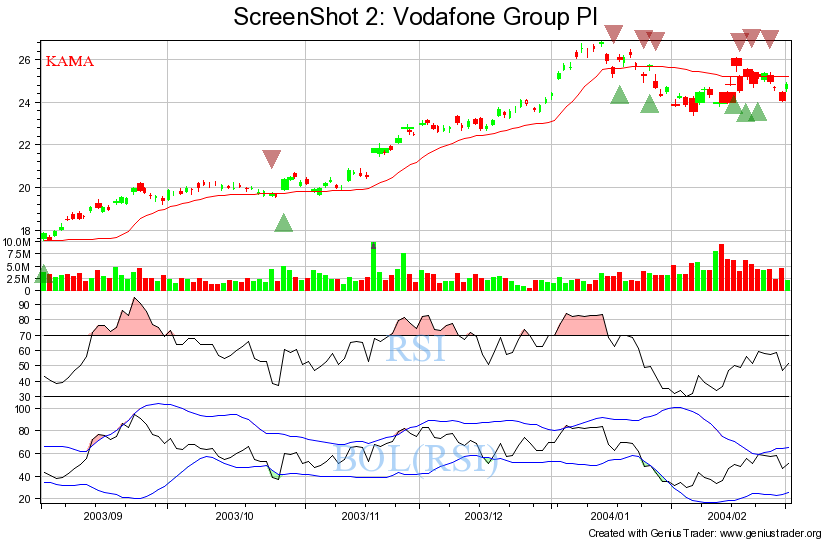
The second screen shot also depicts a day timeframe,
but this price chart uses the volumeplace candles
which incorporate volume in the candle width.
Hard to see in this example, look closely at those
candles on which the trading volume spikes.
The price plot also includes the line curve of
the KAMA indicator (red line) and BuySellArrows based on
the closing price relative to the Systems::Generic sys-sig-indic description.
The arrow colors, size and location may be
adjusted using GT configuration file ($HOME/.gt/options)
and these key-values:
Graphic::BuySellArrows::BuyColor    "[0,135,0,64]"  # very dark green
Graphic::BuySellArrows::SellColor   "[150,0,0,64]"  # dark red
Graphic::BuySellArrows::Distance    24
Graphic::BuySellArrows::SizeFactor  6
The chart also shows additional indicator plots for
RSI and Bollinger Bands which are computed on the RSI.
Note the advanced color highlighting used in the BOL(RSI) plot.
Also pay close attention to the syntactic structure of the GT
I:G:If statement:
I:G:If 'cond' 'then do this' 'else do this'
It's a bit like the trinary operator from 'c' and perl,
but without the syntactic sugar (e.g. the '?' and the ':',
or an explicit 'else').
Not shown in this screenshots sys-sig-indic, but
important to understand when formulating complex systems
and signals, the GT logical signals AND, OR work on the list
of signals in the logic signals group:
{ S:G:And {signal_1} {signal_2} ... {signal_N} }
and
{ S:G:Or {signal_1} {signal_2} ... {signal_N} }
Screen Shot 3 was created with this graphic.pl
command:
$ ./graphic.pl --file screenshot_3.gconf --out 'Screenshot 3.png' SI
where the graphic directives file screenshot_3.gconf
contains these lines:
    #
    # ./graphic.pl --file screenshot_3.gconf --out 'Screenshot 3.png' SI
    #
    --start=2004-09-01
    --end=2005-03-01
    --title=ScreenShot 3: %n
    --type=barchart
    --add=Switch-Zone(0)
    --add=Curve(Indicators::SafeZone/1, [255,0,0])
    --add=Curve(Indicators::SafeZone/2, [255,0,0])
    #--add=Curve(Indicators::VIDYA)
    --add=Text(SafeZone, 6, 90, center, center, small, [255,0,0], times)
    #--add=Text(VIDYA, 6, 80, center, center, small, black, times)
    --add=set-scale(auto)

    --add=Switch-Zone(1)
    --add=Curve(Indicators::SMA 50 {Indicators::Prices VOLUME}, dark blue)
    --add=Text("50 day volume sma", 2, 100, left, center, small, blue, arial)

    --add=New-Zone(6)
    --add=New-Zone(75)
    --add=Curve(Indicators::DSS)
    --add=MountainBand( \
     I:G:Eval min( {I:G:Eval 80}, 100 ),I:G:Eval 100, [180,0,0,100] )
    --add=MountainBand( \
     I:G:Eval min( {I:G:Eval 20}, 0 ),I:G:Eval 20, [0,180,50,100] )
    --add=Text(DSS, 50, 50, center, center, giant, [80,160,240,70], times)

    --add=New-Zone(6)
    --add=New-Zone(75)
    --add=Curve(Indicators::OBV)
    --add=Text(OBV, 50, 50, center, center, giant, [80,160,240,70], times)

    --add=New-Zone(6)
    --add=New-Zone(75)
    --add=Curve(Indicators::RMI 21, 10, {I:OBV})
    --add=Curve(Indicators::Generic::Eval 80,[200,0,0])
    --add=Text(RMI(OBV), 50, 50, center, center, giant, [80,160,240,70], times)
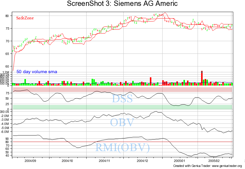
The third screen shot shows the traditional ohlc bar chart along
with a number of other indicators.
Note that the directive to plot VIDYA indicator is commented out.
At this time the VIDYA indicator is not part of the standard GT toolkit,
but might be available via the geniustrader-devel list archive.
This screen shot shows how to select and augment the volume plot
with a 50 day SMA volume curve.
In addition note the usage of MountainBand to shade the
upper and lower extremes of the DSS plot.
scan.pl
reads input data from two file types, a
market file
which is just a list of symbol codes and a
system file
that contains GT sys-sig-indic descriptions defining possible
entry point opportunities.
Recall that a GT System defines two possible signals (entry points),
a long and a short.
A signal is just a single boolean,
so a generic signal must be defined to
denote either a long or a short when used as one-half
of a GT System.Note that a CloseStrategy is also a two signal object,
but must signal exit opportunities.
The first signal still applies to long positions and the second to shorts,
but they typically generate signals that either reduce or close existing
positions.
Note however, GT::CloseStrategy::Reinvest objects are intended to do the
logical opposite, meaning these types of CloseStrategies will actually
increase existing positions.
The following is an example of a GT sys-sig-indic description.
It is a composite generic signal of the six generic below signals
of three SMA indicators with different time span values all
logically anded together.
This signal will trigger when a stock is
consistently falling.
   S:G:And \
     { S:G:Below {I:Prices HIGH } { I:SMA  8 {I:Prices CLOSE} } } \
     { S:G:Below {I:Prices CLOSE} { I:SMA  8 {I:Prices CLOSE} } } \
     { S:G:Below {I:Prices HIGH } { I:SMA 10 {I:Prices CLOSE} } } \
     { S:G:Below {I:Prices CLOSE} { I:SMA 10 {I:Prices CLOSE} } } \
     { S:G:Below {I:Prices HIGH } { I:SMA 12 {I:Prices CLOSE} } } \
     { S:G:Below {I:Prices CLOSE} { I:SMA 12 {I:Prices CLOSE} } } \
   NAME highs and closes below sma 40+50+60day 8+10+12week close sell sell sell
For the scan.pl
examples two input files are necessary, the
market file (./market_file.scan)
contains these three lines:
  AAPL
  IBM
  VOD
The system file (./sys_4.scan) contains these lines:
  # example system_file for screen shot 4
  #
  # todays price close was above open

  S:Generic:Above { I:Prices CLOSE } { I:Prices OPEN }
  # end of system_file
Use scan.pl
to search for a trading signal on a list of codes.
This simple example will report if a stocks price
closes higher than the opening price on 2004-02-01.
The default text output is written to the terminal.
$ ./scan.pl \
--start 2003-08-01 \
--end 2004-02-01 \
./market_file.scan 2004-02-01 ./sys_4.scan
  Signal: S:G:Above {I:Prices CLOSE} {I:Prices OPEN}
   IBM      International Bus
   VOD      Vodafone Group Pl
The same scan.pl
run as in Screen Shot 4 but with option --html.
The output is redirected to the file ./Screenshot_5.html.
$ ./scan.pl --html \
--start 2003-08-01 \
--end 2004-02-01 \
./market_file.scan 2004-02-01 ./sys_4.scan \
> ./Screenshot_5.html
The generated webpage of Screen Shot 5.
backtest.pl
uses a lot of user personalized data files which
make it especially difficult to provide screen shot examples that
will be simple to reproduce. However, we will attempt to describe
where the most likely issues will occur.
In order to provide multiyear examples these examples do
use the GT sample data from here.
Refer to instructions at top of the page for installation detail.
Once again the GT configuration file
$HOME/.gt/options
will be involved, but we will use command line directives
to minimize difficulty. The quoting shown is necessary to
escape certain characters from both the shell and from internal
GT options processing.
Unfortunately backtest.pl
does not [yet] have provisions to read
operating directives from a file, so the command lines are brutal
to type. You can always create a little wrapper script and ''can''
your frequently used backtest.pl commands.
backtest.pl
does not [yet] have a default time frame so
you must pass the
--graph='timeframe name'
option.
backtest.pl
must be passed the
--graph='filename'
option if you want a chart of the analysis,
this is true even if you are generating html output.
The author believes (or may be just clueless)
backtest.pl
will always output to the terminal.
This is just poor implemention and should be corrected.
Unfortunately the task isn't entirely trivial, since
it would be also reasonable to also ensure that the
embedded graphic image url pathname is correct relative
to the html output pathname even when they are specified
inconsistently by the user.
If you are going to be generating html output and
want to include the plot image be sure to specify an
absolute pathname for the graph, that way your browser
or http server will be able to find the image.
Note that your default broker is typically defined in
$HOME/.gt/options
so in that case you can ignore the option
--broker=NoCosts if you want.
The chart image graph line colors denote GT trading system (portfolio) performance in green and the 'buy and hold' performance in red. In the 'History of the portfolio' table the background color denotes winning trades (green) and losing trades (red).
Backtest analysis can be trade intensive,
in order to limit the number of trades in this example we are
using a trivial predefined trading system (TFS) and specify a
weekly timeframe.
backtest.pl
will mark each trade on the chart with the option
--display-trades: note the red/green triangles
and orange line along the bottom of the chart.
Note: there is a ras hack of backtest.pl
(possibly available in the GT devel archive)
that uses the graphic object Positions
to draw buys and sells on the chart
instead of the Trades graphic object to mark
trades alone the bottom axis.
$ ./backtest.pl --option='Graphic::BackgroundColor=White' \ --option='DB::module=Text' \ --option='DB::text::directory=/usr/local/src/genius_trader/sample_data' \ --graph=/tmp/Screenshot_6.png \ --timeframe week \ --display-trades \ --html \ --broker=NoCosts \ TFS 13000 > /tmp/Screenshot_6.html
The generated webpage Screen Shot 6.
This backtest.pl example uses the predefined GT system TFS. It changes none of the default arguments and accepts the built-in defaults for closestrategy (TFS) and money-management (Basic). Note although backtest.pl uses the default GT closestrategy TFS. This selection isn't a consequence of the TFS system. The implication is GT Systems do not provide exit signals (CloseStrategy). The complete trading system description is shown at the top of the output report.
$ ./backtest.pl --option='Graphic::BackgroundColor=White' \ --option='DB::module=Text' \ --option='DB::text::directory=/usr/local/src/genius_trader/sample_data' \ --timeframe day \ --html \ --full \ --graph=/tmp/Screenshot_7.png \ --broker=NoCosts \ TFS 13000 > /tmp/Screenshot_7.html
The generated webpage Screen Shot 7.
Use backtest.pl, the sample data for cusip code 13000 (Alcatel) with the command line arguments shown below to generate the html output depicted in Screenshot 8.
You have to enter the long quoted strings as shown,
meaning without attempting to continue the --system or --close-strategy
sys-sig-indic descriptions, because the shell will not reassemble
the quoted string before passing it on to the perl interpreter.
Yet another reason to use a little wrapper script for
frequently used commands.
$ ./backtest.pl --option='Graphic::BackgroundColor=White' \
--start=1993-01-04 \
--end=2004-03-08 \
--system='Generic {S:Generic:CrossOverUp {I:DMI/3 14} 12} {S:Generic:CrossOverDown {I:DMI/3 14} -12}' \
--close-strategy='Generic {S:Generic:CrossOverDown {I:DMI/3 14} 12} {S:Generic:CrossOverUp {I:DMI/3 14} -12}' \
--money-management="Basic" \
--html \
--timeframe day \
--graph=/tmp/Screenshot_8.png \
13000 > /tmp/Screenshot_8.html
The generated webpage Screen Shot 8.
backtest_many.pl implements reading input data from files specified on the comand line. So backtest_many.pl can ease some of the command line anguish caused by backtest.pl not reading input files. These input file arguments must appear on the comamnd line, if they are not found stdin will be read without prompting of any kind. The files must be in this order:
   market_file -=- lists stock codes, one code per line
   system_file -=- lists one or more GT trading systems descriptions

  $  ./backtest_many.pl [ options ] market_file system_file [ system_file ... ]
In addition backtest_many.pl can be used to evaluate multiple GT trading systems, refer to the pod manual (perldoc -t backtest_many.pl).
The market_file can be shared with scan.pl However, because scan.pl parses GT trading systems more like a pair of signals you will have trouble trying to use the same system_file with both scan.pl and backtest_many.pl.
to be provided